Plot method for object of class decontaminated_density

Plot the decontaminated density of the unknown component from some admixture model, after inversion of the admixture cumulative distribution functions.

Usage

# S3 method for class 'decontaminated_density'
plot(
  x,
  x_val = NULL,
  add_plot = FALSE,
  offset = 0,
  bar_width = 0.3,
  main = "pdf of the unknown component",
  ...
)

Arguments

x

An object of class decontaminated_density (see ?decontaminated_density).

x_val

Values at which to evaluate the decontaminated density.

add_plot

Boolean, TRUE when a new plot is added to the existing one.

offset

Numeric. Position of the bars relative to the labels on the x-axis.

bar_width

Width of bars to be plotted.

main

The title of the plot (typically 'probability density function of the unknown component', or 'probability mass function of the unknown component').

...

Arguments to be passed to generic method plot, such as graphical parameters (see ?par).

Value

The plot of the decontaminated density if one sample is provided, or the comparison of decontaminated densities plotted on the same graph in the case of multiple samples.

Details

The decontaminated density is obtained by inverting the admixture density, given by l = p*f + (1-p)*g, to isolate the unknown component f after having estimated p and l.

Author

Xavier Milhaud xavier.milhaud.research@gmail.com

Examples

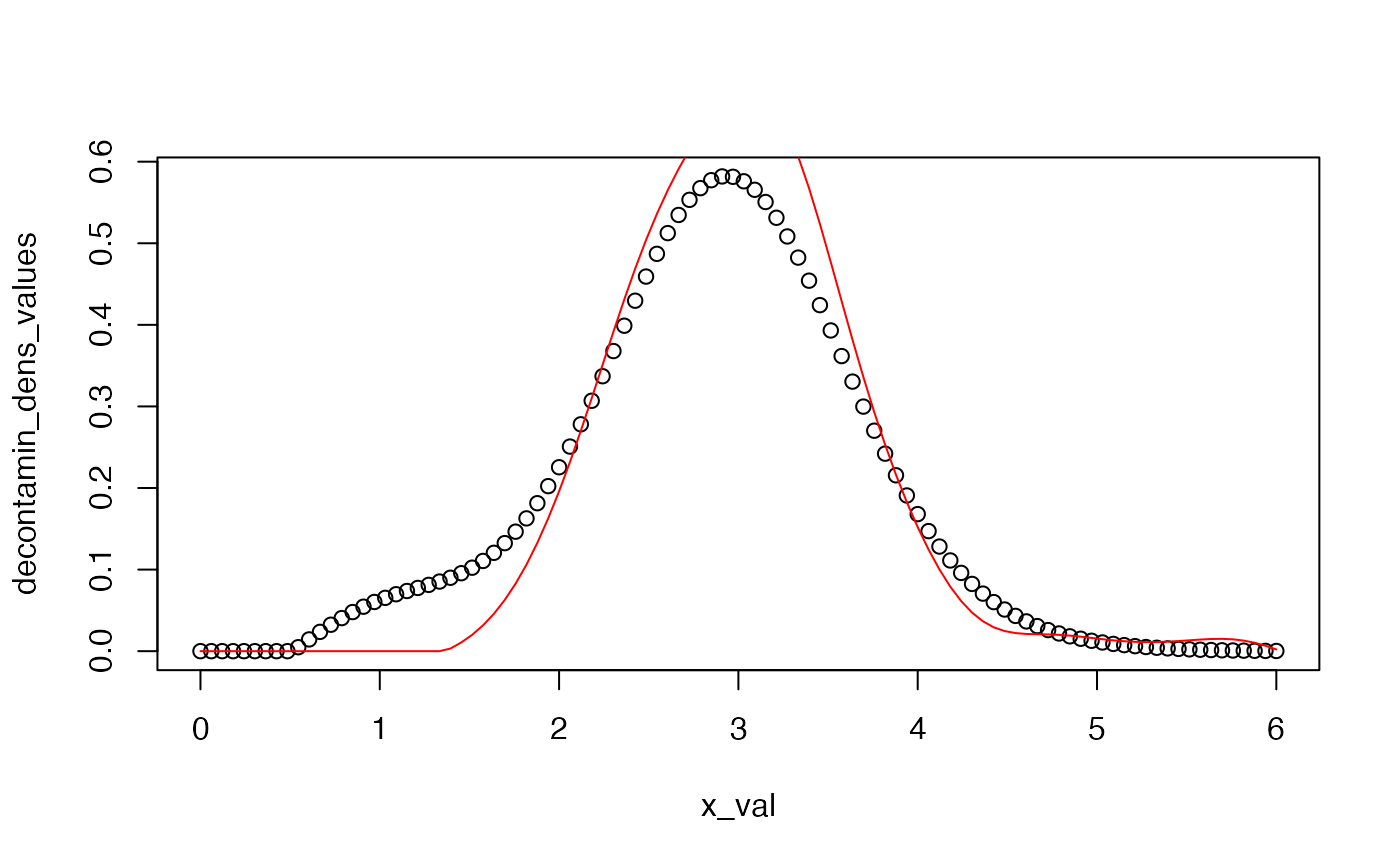
## Simulate mixture data:
mixt1 <- twoComp_mixt(n = 400, weight = 0.4,
                      comp.dist = list("norm", "norm"),
                      comp.param = list(list("mean" = -2, "sd" = 0.5),
                                        list("mean" = 0, "sd" = 1)))
data1 <- get_mixture_data(mixt1)
## Define the admixture models:
admixMod1 <- admix_model(knownComp_dist = mixt1$comp.dist[[2]],
                         knownComp_param = mixt1$comp.param[[2]])
## Estimation:
est <- admix_estim(samples = list(data1), admixMod = list(admixMod1),
                   est_method = 'PS')
## Determine the decontaminated version of the unknown density by inversion:
x <- decontaminated_density(sample1 = data1, admixMod = admixMod1,
                            estim.p = get_mixing_weights(est))
plot(x)


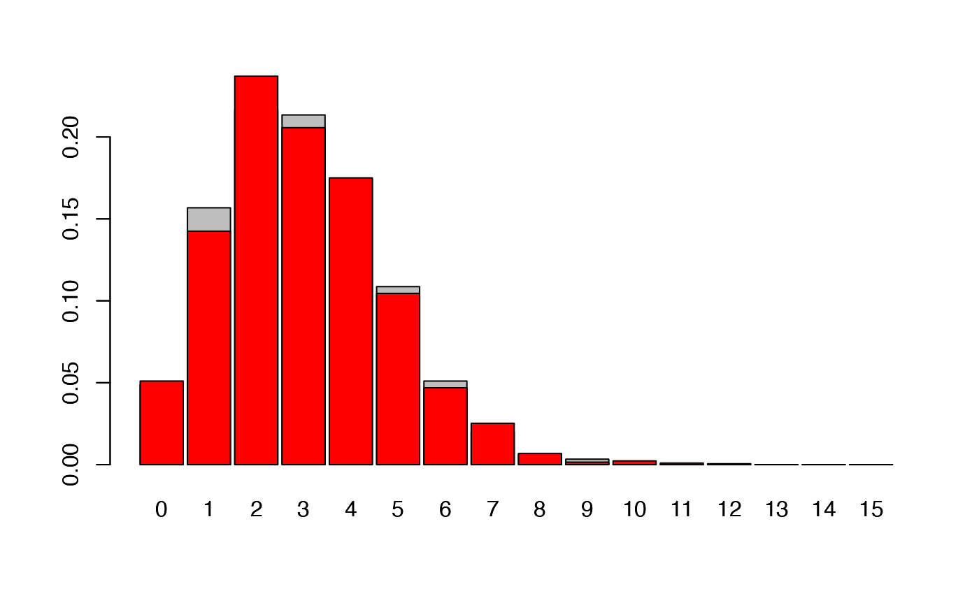
####### Discrete support:
mixt1 <- twoComp_mixt(n = 4000, weight = 0.6,
                      comp.dist = list("pois", "pois"),
                      comp.param = list(list("lambda" = 3),
                                        list("lambda" = 2)))
mixt2 <- twoComp_mixt(n = 3000, weight = 0.8,
                      comp.dist = list("pois", "pois"),
                      comp.param = list(list("lambda" = 3),
                                        list("lambda" = 4)))
mixt3 <- twoComp_mixt(n = 1500, weight = 0.5,
                      comp.dist = list("pois", "pois"),
                      comp.param = list(list("lambda" = 7),
                                        list("lambda" = 1)))
data1 <- get_mixture_data(mixt1)
data2 <- get_mixture_data(mixt2)
data3 <- get_mixture_data(mixt3)
## Define the admixture models:
admixMod1 <- admix_model(knownComp_dist = mixt1$comp.dist[[2]],
                         knownComp_param = mixt1$comp.param[[2]])
admixMod2 <- admix_model(knownComp_dist = mixt2$comp.dist[[2]],
                         knownComp_param = mixt2$comp.param[[2]])
admixMod3 <- admix_model(knownComp_dist = mixt3$comp.dist[[2]],
                         knownComp_param = mixt3$comp.param[[2]])
## Estimation:
est <- admix_estim(samples = list(data1,data2),
                   admixMod = list(admixMod1,admixMod2), est_method = 'IBM')
#>  IBM estimators of two unknown proportions are reliable only if the two corresponding
#>  unknown component distributions have previously been tested equal (see ?admix_test).
est2 <- admix_estim(samples = list(data3), admixMod = list(admixMod3), est_method = 'PS')
## Determine the decontaminated version of the unknown density by inversion:
x <- decontaminated_density(sample1 = data1, admixMod = admixMod1,
                            estim.p = get_mixing_weights(est)[1])
y <- decontaminated_density(sample1 = data2, admixMod = admixMod2,
                            estim.p = get_mixing_weights(est)[2])
z <- decontaminated_density(sample1 = data3, admixMod = admixMod3,
                            estim.p = get_mixing_weights(est2))
plot(x, offset = -0.2, bar_width = 0.2, main = "pmf of the unknown component", col = "steelblue")
plot(y, add_plot = TRUE, offset = 0, bar_width = 0.2, col = "red")
plot(z, add_plot = TRUE, offset = 0.2, bar_width = 0.2, col = "orange")
legend("topright", legend = c("data1","data2","data3"), col = c("steelblue","red","orange"),
       lty = rep(1,3), lwd = rep(2,3), bty = "n")